The LHCb experiment at CERN used to have a straw tube detector in the main tracker. It consists of modules of circular straws of 5 mm diameter with a metalized wall and an anode wire in the middle:
                                          #####
     /              /                    #     #
    +--------------+                    #   *   #
    |O O O ... O O |                     #     #
    | O O O ... O O|/                     #####
    +--------------+                cross section of straw
cross section of module             * anode wire
O - straw
The modules were 5 m long, and consisted of 2 monolayers of straws 5.25 mm apart (pitch), with the second monolayer offset by half the pitch. An electrical potential (around 1450 V) was applied between anode wire and straw wall, and straws were filled with a counting gas (Ar/CO₂/O₂ 70/28.5/1.5%).
  ##### /    / charged particle
 #     #     # straw wall
#   * / #    * anode wire
 #   / #
  #####
   /
When a charged particle traverses a straw, it ionises the counting gas, and the resulting charges are accelerated in the electical field. When they reach the region around the anode wire, they create an avalanche-like charge amplification in the strong field close to the wire, resulting in signal amplification. The resulting charge pulse is registered in the front end electronics when it rises above a certain threshold, and the arrival time is registed with a TDC (time-to-digital converter). Since the arrival time of the particles is known from the LHC clock and known time of flight to the detector, it is possible to work out the drift time, and obtain around 200 µm spatial resolution for the distrance between particle and anode wire.
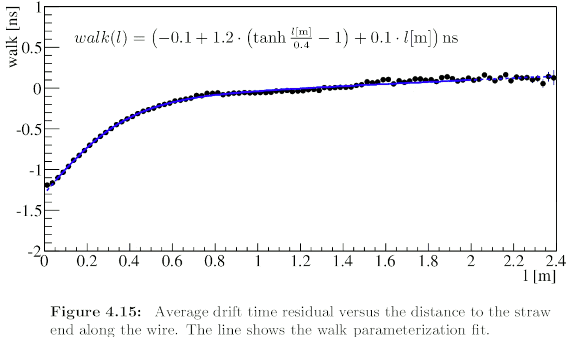
To work out the drift time, various corrections need to be applied, among them the so-called time walk correction:
The TDC measures the arrival time of the charge pulse, which is taken as the time at which the readout signal rises above a threshold. But the signal is attenuated by travel along the anode wire. This means that more strongly attenuated signals rise above threshold a bit later, giving rise to a correction that depends on the length along the straw (as seen from the readout).
A typical example can be taken from Alexandr Vladimirovich Kozlinskiy’s PhD thesis (Amsterdam, 2013):
The data can be described well with the tanh function.
The time walk correction was put into LHCb reconstruction software. After the change, the LHCb trigger farm which has to process detector data in near real-time to decide which data to keep for writing to tape and which data to discard suddenly spent 30% of CPU on calculating tanh instead of the rest of event reconstruction. This directly translates to a 30% loss in experiment statistics for as long as the situation persists.
Clearly, some optimization was needed, and a lookup table was quickly deployed, and solved the immediate problem.
While a lookup table is an easy solution, there are better ones. The idea is to look into some of them.
One crucial question when approximating a function is how accurate the approximation should be.
In our case, there are two natural scales: The LHCb Outer Tracker front end electronics contains a TDC with 391 ps resolution. The statistical nature of particle drift means that the intrinsic uncertainty in particle arrival times at a given radius from the anode wire is around 1 ns (so the TDC is somewhat overdesigned).
That means that as long as we stay about one order of magnitude below the 1 ns limit with the approximation, we are unlikely to see in the data that tanh was replaced with an approximation.
The simplest thing one can try is a Taylor series. Since we want to compete with a lookup table in terms of speed, we cannot go to very high orders.
tanh(x) ≈ 𝑥 − 𝑥³/3 + 2/15 𝑥⁵ − 17/315 𝑥⁷ + 62/2835 𝑥⁹ − 1382/155925 𝑥¹¹
        + 21844/6081075 𝑥¹³ − 929569/638512875 𝑥¹⁵
Implement a Taylor series in the programming language of your choice.
How accurate is it?
How fast is it? (Hint: measure how long it takes to calculate tanh and the approximation on 1 M random numbers.)
In Python, use something like:
import time

start = time.perf_counter()
do_sth() # whatever needs to be timed
end = time.perf_counter()

print("elapsed time: {} s".format(end - start))
In C++, the corresponding code is:
#include <chrono>

const auto start{std::chrono::high_resolution_clock::now()};
do_sth(); // whatever needs to be timed
const auto finish{std::chrono::high_resolution_clock::now()};
const std::chrono::duration<double> elapsed{finish - start};
double time_in_seconds = elapsed.count();
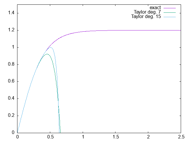
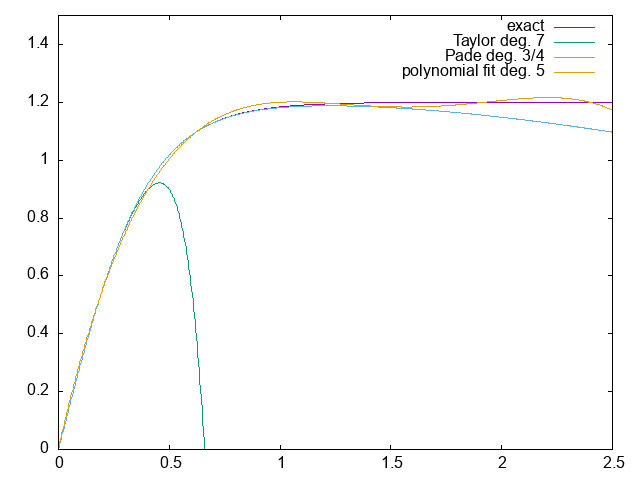
The “exact” function plotted is 1.2 tanh(x / 0.4), so the unit on the x axis is metres and ns on the y axis, so results can be compared to the original time walk correction plot.
You can of course use whatever function plotting package you like (ROOT, matplotlib, … are all okay). I often find myself going for gnuplot for simple function visualisation because it’s quick and easy (most plots today were made with gnuplot):
# gnuplot

        G N U P L O T
        Version 5.4 patchlevel 4    last modified 2022-07-10

        Copyright (C) 1986-1993, 1998, 2004, 2007-2022
        Thomas Williams, Colin Kelley and many others

        gnuplot home:     http://www.gnuplot.info
        faq, bugs, etc:   type "help FAQ"
        immediate help:   type "help"  (plot window: hit 'h')

Terminal type is now 'wxt'
gnuplot> f_t(x)=x-x**3/3.+2*x**5/15.-17*x**7/315.
gnuplot> plot [0:2.5] [0:1.5] 1.2*tanh(x/0.4) t 'exact', 1.2*f_t(x/0.4) t 'Taylor deg. 7'
gnuplot> quit
A Padé approximant is a ratio of polynomials. The coefficients are chosen such that the Taylor series of the ratio matches that of the function to be approximated for a number of terms.
For example, up to 𝑥⁷, we have
tanh(x) ≈ 𝑥 − 𝑥³/3 + 2/15 𝑥⁵ − 17/315 𝑥⁷
P(x)    = (10 𝑥³ + 105 𝑥) / (𝑥⁴ + 45 𝑥² + 105)
        ≈ 𝑥 − 𝑥³/3 + 2/15 𝑥⁵ − 17/315 𝑥⁷
(Padé approximants are typically derived using computer algebra systems such as Maxima or Mathematica, but if you know your algebra and calculus, you can code up your own routine as well…)
Visualize P(x). How accurate is it?
How fast is it?
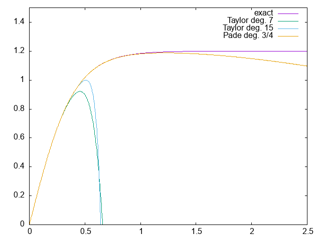
The “exact” function plotted is 1.2 tanh(x / 0.4), so the unit on the x axis is metres and ns on the y axis, so results can be compared to the original time walk correction plot.
Computer algebra systems like Maxima (free software) can help finding Padé approximants:
# maxima

Maxima 5.46.0 https://maxima.sourceforge.io
using Lisp GNU Common Lisp (GCL) GCL 2.6.14 git tag Version_2_6_15pre3
Distributed under the GNU Public License. See the file COPYING.
Dedicated to the memory of William Schelter.
The function bug_report() provides bug reporting information.
(%i1) t:taylor(tanh(x), x, 0, 7);
                              3      5       7
                             x    2 x    17 x
(%o1)/T/                 x - -- + ---- - ----- + . . .
                             3     15     315
(%i2) p:pade(t,3,4);
                                    3
                                10 x  + 105 x
(%o2)                         [----------------]
                                4       2
                               x  + 45 x  + 105
Sometimes, there are helpful identities for the function that needs to be approximated. For example,
𝑡𝑎𝑛h(2𝑥) = 2 𝑡𝑎𝑛h(𝑥) / (1 + 𝑡𝑎𝑛h²(𝑥))
Can you see how that is helpful?
Write an approximation based on this idea. How accurate is it?
How fast is it?
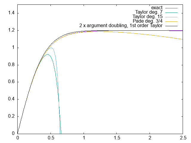
The “exact” function plotted is 1.2 tanh(x / 0.4), so the unit on the x axis is metres and ns on the y axis, so results can be compared to the original time walk correction plot.
Adapt yesterday’s fitting code to fit a polynomial to the walk relation.
Visualize the results. How accurate is it?
How fast is it?
The “exact” function plotted is 1.2 tanh(x / 0.4), so the unit on the x axis is metres and ns on the y axis, so results can be compared to the original time walk correction plot.
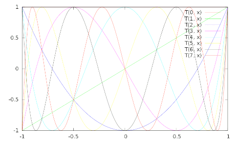
Chebyshev polynomials are defined on the interval 𝑥 ∈ [−1, +1]:
𝑇₀(𝑥) = 1     𝑇₁(𝑥) = 𝑥     𝑇ₙ(𝑥) = 2𝑥 𝑇ₙ₋₁(𝑥) − 𝑇ₙ₋₂(𝑥)

𝑇ₙ(𝑥) = 𝑐𝑜𝑠(𝑛 𝑎𝑐𝑜𝑠(𝑥))
Adapt yesterday’s fitting code to fit a Chebyshev series to the walk relation.
Visualize the results. How accurate is it?
How fast is it?
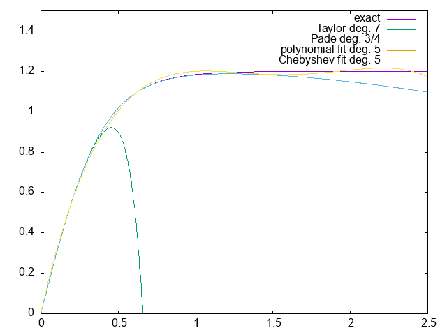
The “exact” function plotted is 1.2 tanh(x / 0.4), so the unit on the x axis is metres and ns on the y axis, so results can be compared to the original time walk correction plot.
Note how the polynomial and Chebyshev fits are right on top of each other – not really surprising considering both have monomials up to 𝑥⁴.
Given how similar polynomial and Chebyshev fits look, you may wonder which one to prefer. Here are the correlation matrices for both:
[  1                       ]     [ 1                     ]
[  0      1                ]     [ 0                     ]
[ -0.745  0 1              ]     [ 0.487 0     1         ]
[  0     -0.917  0     1   ]     [ 0     0.420 0     1   ]
[  0.601  0     -0.959 0 1 ]     [ 0.235 0     0.381 0 1 ]

correlations: polynomial fit     correlations: Chebyshev fit
While the exact values tend to depend on number and spacing of measurements, and on uncertainties, Chebyshev polynomial fits tend to be more stable due to smaller correlations.
Running today’s examples in C++ and python, we can work out how long a loop running over 1M values needs per iteration (on my laptop):
| function | C++ [ns] | Python [ns] |
|---|---|---|
| tanh | 49.0 | 123.1 |
| taylor7 | 12.0 | 405.6 |
| pade34 | 5.6 | 428.9 |
| dbl2 | 11.0 | 624.4 |
| poly fit | 7.4 | 244.0 |
| cheby fit | 10.9 | 934.8 |
Clearly, these numbers have to be taken with a grain of salt (the laptop is old, and was running other things as well).
| function | C++ [ns] | Python [ns] |
|---|---|---|
| tanh | 49.0 | 123.1 |
| taylor7 | 12.0 | 405.6 |
| pade34 | 5.6 | 428.9 |
| dbl2 | 11.0 | 624.4 |
| poly fit | 7.4 | 244.0 |
| cheby fit | 10.9 | 934.8 |
However, there are a couple of observations one might make: