Here’s what’s on the menu today:
Assume: - you have N uncorrelated measurements - the measured values 𝑥ᵢ are normally distributed around the true value of 𝑥 with uncertainty σᵢ
We can write the probability density function (PDF) to find each measurement 𝑥ᵢ given the true value 𝑥 as
             _____
𝑃(𝑥ᵢ|𝑥) = 1/√2πσᵢ² 𝑒𝑥𝑝(−(𝑥ᵢ − 𝑥)²/2σᵢ²)
Clearly, the combined likelihood for all measurements is
ℒ = ∏ ᵢ 𝑃(𝑥ᵢ|𝑥)
We are looking for an estimate of the true value 𝑥, 𝔵, at which the likelihood has a maximum. As the likelihood is a fast changing function, it is easier (numerically) to look for a minimum in −𝑙𝑛 ℒ.
A necessary condition for a minimum is 𝜕/𝜕𝔵 (−𝑙𝑛 ℒ) = 0.
−𝑙𝑛 ℒ = 𝑐𝑜𝑛𝑠𝑡. + ∑ ᵢ (𝑥ᵢ − 𝔵)²/2σᵢ²
We drop the constant (which is from the normalisation factors of the PDFs of the individual measurements) because it drops out in the derivative (does not depend on 𝔵).
The remaining sum is important enough to have its own Greek letter:
χ² = ∑ ᵢ (𝑥ᵢ − 𝔵)²/2σᵢ²
χ² = ∑ ᵢ (𝑥ᵢ − 𝔵)²/2σᵢ²
This is the key ingredient of the method of least squares. One forgets about the precise shape of the measurement PDFs, and as long as there are a handful of measurements, this method will yield good results due to the central limit theorem. (Gauss already knew this!)
Grab pen and paper, and do the derivative!
𝜕χ² / 𝜕𝔵 =
Grab pen and paper, and do the derivative!
0 = 𝜕χ²/ 𝜕𝔵 = ∑ ᵢ 𝜕/𝜕𝔵 (𝑥ᵢ − 𝔵)² / 2σᵢ²

            = ∑ ᵢ 2(𝑥ᵢ − 𝔵)/2σᵢ²

            = ∑ ᵢ 𝑥ᵢ/σᵢ² − ∑ ᵢ 𝔵/σᵢ²
Or:
∑ ᵢ 𝑥ᵢ/σᵢ² = 𝔵 ⋅ ∑ ᵢ 1/σᵢ²
∑ ᵢ 𝑥ᵢ/σᵢ² = 𝔵 ⋅ ∑ ᵢ 1/σᵢ²
At this point, we introduce some abbreviations: For a per-measurement quantity 𝑞, we write
⟨𝑞⟩ = ∑ ᵢ 𝑞ᵢ/σᵢ²
With this, the equation on top becomes:
⟨𝑥⟩ = 𝔵 ⋅ ⟨1⟩
Or
𝔵 = ⟨𝑥⟩ / ⟨1⟩
Hah, that was easy!
Say you have a resistance which is a bit tricky to measure (a small resistor below 1 Ω), which you need to measure several times, and you decide to average the measurements:
| measurement number | 1 | 2 | 3 |
|---|---|---|---|
| R [Ω] | 0.5 | 0.2 | 0.3 |
| σ [Ω] | 0.25 | 0.1 | 0.1 |
What’s the best guess for the true resistance of R? What’s its expected uncertainty? (hint: What χ² would you get for a single Gaussian PDF?)
Write a little computer program that does the calculation.
#!/usr/bin/env python3
#
# day1-ex1.py - weighted mean and error of uncorrelated measurements
import math

Rs =     [  0.5, 0.2, 0.3 ]
sigmas = [ 0.25, 0.1, 0.1 ]

def calc_weighted_mean_and_err(xs, sigmas):
    sum_x = 0
    sum_1 = 0
    for xi, sigmai in zip(xs, sigmas):
        w = 1 / (sigmai * sigmai)
        sum_x += w * xi
        sum_1 += w

    return sum_x / sum_1, math.sqrt(1 / sum_1)


print("weighted mean of {} measurements is {} +/- {}".format(
        len(Rs), *calc_weighted_mean_and_err(Rs, sigmas)))
Often, your scenario is a bit more complex: You have measurements, but your measurement device is imperfect, and you need to calibrate it with a set of reference measurements. In the simplest case, the relationship between the true value 𝔵 and your measurement x is linear, e.g.
𝑥 = 𝑎 ⋅ 𝔵 + 𝑏
The parameters 𝑎 and 𝑏 need to be determined during the calibration procedure. Let’s say we want to calibrate a volt meter with a set of voltage references:
| measurement number | 1 | 2 | 3 | 4 |
|---|---|---|---|---|
| reference 𝔵 (true) [V] | 0 | 1 | 2 | 5 |
| measured 𝑥 [V] | 0.09 | 1.05 | 1.72 | 4.15 |
The uncertainty for all measured voltages is 0.1 V.
Given the model from the last slide,
𝑥 = 𝑎 ⋅ 𝔵 + 𝑏
the χ² function comes out as
χ² = ∑ ᵢ (𝑥ᵢ − a𝔵 − 𝑏)²/2σᵢ²
We need to minimize that function with respect to the fit parameters 𝑎 and 𝑏.
χ² = ∑ ᵢ (𝑥ᵢ − a𝔵ᵢ − 𝑏)²/2σᵢ²
Putting the derivatives to zero yields:
0 = 𝜕χ²/𝜕𝑎 = ∑ ᵢ (𝑥ᵢ − 𝑎𝔵ᵢ − 𝑏)(-𝔵) / σᵢ²
0 = 𝜕χ²/𝜕𝑏 = ∑ ᵢ (𝑥ᵢ − 𝑎𝔵ᵢ − 𝑏)(-1) / σᵢ²
Or, in terms of our “shorthand”,
𝑎 ⟨𝔵²⟩ + 𝑏 ⟨𝔵⟩ = ⟨𝑥𝔵⟩
𝑎 ⟨𝔵 ⟩ + 𝑏 ⟨1⟩ = ⟨𝑥 ⟩
Or, in matrix form (let’s call the matrix below M):
/ ⟨𝔵²⟩ ⟨𝔵⟩ \ / a \  =  / ⟨𝑥𝔵⟩ \
\  ⟨𝔵⟩ ⟨1⟩ / \ b /     \ ⟨𝑥 ⟩ /
Let’s stick with our example of calibrating a Volt meter with a linear function.
| measurement number | 1 | 2 | 3 | 4 |
|---|---|---|---|---|
| reference 𝔵 (true) [V] | 0 | 1 | 2 | 5 |
| measured 𝑥 [V] | 0.09 | 1.05 | 1.72 | 4.15 |
The uncertainty for all measured voltages is 0.1 V.
Code up a short program that fits a straight line to the data, outputs the fit paramters, and their uncertainties and correlation matrix.
#!/usr/bin/env python3
#
# day1-ex2.py - straight line fit

import math

def invert2x2(m):
    """ invert 2x2 matrix - we should use something better here! """
    det = m[0][0] * m[1][1] - m[0][1] * m[1][0]
    return [[m[1][1] / det, -m[1][0] / det],
            [-m[0][1] / det, m[0][0] / det]]


def mulM2x2V(m, v):
    """ multiply a 2x2 matrix with a two element vector """
    return [m[0][0] * v[0] + m[0][1] * v[1], m[1][0] * v[0] + m[1][1] * v[1]]
def fitStraightLine(xs, ys, sigmas):
    """ fit a straight line to given data points """
    mat = [[0, 0], [0, 0]]
    rhs = [0, 0]
    for x, y, sigma in zip(xs, ys, sigmas):
        w = 1 / (sigma * sigma)
        rhs[0] += w * y * x
        rhs[1] += w * y
        mat[0][0] += w * x * x
        mat[0][1] += w * x
        mat[1][1] += w
    mat[1][0] = mat[0][1]
    cov = invert2x2(mat)
    sol = mulM2x2V(cov, rhs)
    return sol, cov
Vtrue = [0, 1, 2, 5]
V = [.09, 1.05, 1.72, 4.15]
sigmas = [.1, .1, .1, .1]

sol, cov = fitStraightLine(Vtrue, V, sigmas)

print("Solution: fit parameters a={} +/- {}".format(sol[0],
                                                    math.sqrt(cov[0][0])))
print("Solution: fit parameters b={} +/- {}".format(sol[1],
                                                    math.sqrt(cov[1][1])))
print("Correlation matrix:")
print("[ {}, {} ]".format(1, cov[0][1] / math.sqrt(cov[0][0]*cov[1][1])))
print("[ {}, {} ]".format(cov[1][0] / math.sqrt(cov[0][0]*cov[1][1]), 1))
What is the covariance matrix?
You know about mean and variance of a scalar quantity 𝑥 (𝔼 denotes the expectation value):
μ(𝑥) = 𝔼(𝑥)
𝑉(x) = 𝔼((𝑥 − 𝔼(𝑥))²)
It’s possible to do the same thing for vector-valued 𝐱∶
𝛍(𝐱)   = 𝔼(𝐱)
𝐶ᵢⱼ(𝐱) = 𝔼((𝐱ᵢ − 𝔼(𝐱ᵢ)) ⋅ (𝐱ⱼ − 𝔼(𝐱ⱼ)))
So the covariance is the matrix that corresponds to the variance if you have a random vector 𝐱 instead of a scalar.
The inverse of the matrix M we get when we minimize χ² is the covariance matrix.
Let’s look at a multivariate Gaussian. The probability to observe a vector 𝐯 with n elements, given the true value is 𝐰 and the covariance is 𝐶, is:
            _____________
𝑃(𝐯|𝐰) = 1/√{(2π)ⁿ 𝑑𝑒𝑡(𝐶)⋅ 𝑒𝑥𝑝(−(𝐯 − 𝐰)ᵀ 𝐶⁻¹ (𝐯 − 𝐰) / 2)
If you go through the motions, and derive χ², you will get
χ² = −(𝐯 − 𝐰)ᵀ 𝐶⁻¹ (𝐯 − 𝐰) / 2
And if you compare that to our straight line fit χ², you see that our matrix M is just the inverse of C.
For now, we have talked a lot about the covariance matrix. Often, you’re stuck with correlations between components of your solution vector, though. Fortunately, the relationship is an easy one:
Covariance matrix 𝐶:                        entries 𝐶ᵢⱼ
                                             ___
uncertainty of component 𝑖:                 √𝐶ᵢᵢ
                                                   ___________
correlation ρᵢⱼ between components 𝑖 and 𝑗: 𝐶ᵢⱼ / √ 𝐶ᵢᵢ ⋅ 𝐶ⱼⱼ
Now, if you have the uncertainties and correlations, you can build a covariance matrix, and vice-versa.
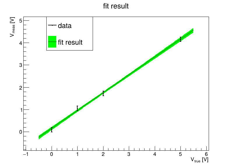
In order to judge the fit, we should visualize our data and fit results:
You can use the software package of your choice (e.g. matplotlib in python). Your choice is fine if you get it to work.
I will use ROOT (data analysis package used extensively in High Energy Physics), because it neatly bridges the C/C++ and Python worlds, something which can come in very useful indeed if you need a bit more speed…
At 𝔵 = 0, the uncertainty of 𝑥 is
σ²(𝑥) = 𝐶₁₁ = σ²(b) at 𝔵 = 0
To transport the uncertainty to other values of 𝔵, let’s look at our model again:
𝑥(𝔵) = 𝑎 𝔵 + 𝑏 = (𝔵 1) / 𝑎 \ = 𝑇(𝔵) / 𝑎 \
                       \ b /        \ b /
The matrix 𝑇(𝔵) is called the transport matrix. It also transforms the covariance matrix:
σ²(𝑥(𝔵)) = 𝑇(𝔵) 𝐶 𝑇ᵀ(𝔵)
(If you want the uncertainty of something that’s a non-linear function of the fit parameters, it’s possible to linearise the formula, and use the Jacobian as transport matrix over small distances.)
#!/usr/bin/env python3
#
# day1-ex3.py - straight line fit results

import math
import ROOT

Vtrue = [0, 1, 2, 5]
V = [.09, 1.05, 1.72, 4.15]
sigmas = [.1, .1, .1, .1]

fitparams = [0.8014, 0.1496]
fitcov = [[0.02673 * 0.02673, -0.7303 * 0.02673 * 0.07319],
          [-0.7303 * 0.02673 * 0.07319, 0.07319 * 0.07319]]

c = ROOT.TCanvas("c", "c", 800, 600)
# build graph for fit result (and uncertainty)
gfit = ROOT.TGraphErrors(100)
gfit.SetNameTitle("gfit", "fit result;V_{true} [V];V_{meas} [V]")
for i in range(0, 121):
    x = Vtrue[3] * (i - 10) / 100.  # range to extend a bit beyond data points
    gfit.SetPoint(i, x, fitparams[0] * x + fitparams[1])
    tmp = [fitcov[0][0] * x + fitcov[0][1], fitcov[1][0] * x + fitcov[1][1]]
    err2 = tmp[0] * x + tmp[1]
    gfit.SetPointError(i, 0., math.sqrt(err2))
gfit.SetLineColor(ROOT.kGreen + 2)
gfit.SetFillColor(ROOT.kGreen)
gfit.SetMarkerColor(ROOT.kGreen + 2)
gfit.SetMarkerSize(0)
gfit.SetLineWidth(2)
# build graph with data
gdata = ROOT.TGraphErrors(len(Vtrue))
gdata.SetNameTitle("gdata", "data")
for i in range(0, len(Vtrue)):
    gdata.SetPoint(i, Vtrue[i], V[i])
    gdata.SetPointError(i, 0., sigmas[i])
gdata.SetLineWidth(2)
gdata.SetMarkerStyle(7)
gdata.SetMarkerSize(2)

gfit.Draw("A3")  # draw axes, and error band
gfit.Draw("LX")  # draw fitted line (without error bars/bands)
gdata.Draw("P")  # draw data

c.SaveAs("day1-ex3.pdf")
You’ve seen the plot, and you’ve seen the correlation between fit parameters 𝑎 and 𝑏 is around -73%. That seems kind of large. Is there a way around it?
The key is to “shift” the place at which the fit parameters are valid. Let’s modify the model a bit:
𝑥(𝔵) = 𝑎 (𝔵 − 𝔵₀) + 𝑏 = 𝑎 𝑑𝔵 + 𝑏
We thus shift the fit parameters to 𝔵₀.
𝑥(𝔵) = 𝑎 (𝔵 − 𝔵₀) + 𝑏 = 𝑎 𝑑𝔵 + 𝑏
Let’s go through the motions, write down χ², work out the derivatives, and put it in matrix form:
χ² = ∑ ᵢ (𝑥ᵢ − a d𝔵ᵢ − 𝑏)²/2σᵢ²

/ ⟨d𝔵²⟩ ⟨d𝔵⟩ \ / a \  =  / ⟨𝑥 d𝔵⟩ \
\  ⟨d𝔵⟩  ⟨1⟩ / \ b /     \ ⟨𝑥   ⟩ /
The correlations is driven by the off-diagonal elements of the matrix, i.e. ⟨d𝔵⟩. How small can we make it?
⟨d𝔵⟩ = ∑ ᵢ (𝔵ᵢ − 𝔵₀) / σᵢ² = ⟨𝔵⟩ - 𝔵₀⋅⟨1⟩
We can actually make this zero, so the optimal choice is 𝔵₀ = ⟨𝔵⟩ / ⟨1⟩. In pactice, this is somewhere in the middle of the data points.
Modify the straight line fit code and visualization examples to use this “shifted” definition of fit parameters.