AI-assisted Python Coding

Day 5: Pandas, scikit-learn, and good coding practices

Klaus Reygers

Studierendentage Physik, Uni Heidelberg, 23.-27.03.2026

Very short introduction to pandas

pandas is a Python library for working with structured (tabular) data.

Quick reference: https://pandas.pydata.org/docs/user_guide/10min.html

Think of it as:

spreadsheet-like tables, but in Python
reproducible and automatable workflows
fast tools for cleaning, transforming, and analyzing data

Core objects: Series and DataFrame

import pandas as pd

s = pd.Series([1.2, 1.5, 1.4], name="voltage")
df = pd.DataFrame({
  "time_s": [0, 1, 2],
  "voltage_V": [1.2, 1.5, 1.4]
})

s, df

(0    1.2
 1    1.5
 2    1.4
 Name: voltage, dtype: float64,
    time_s  voltage_V
 0       0        1.2
 1       1        1.5
 2       2        1.4)

Series: one labeled column
DataFrame: labeled 2D table

Create and inspect a DataFrame

df = pd.DataFrame({
  "x": [1, 2, 3, 4, 5],
  "y": [1.7, 2.3, 3.5, 3.3, 4.3],
  "sigma_y": [0.5, 0.3, 0.4, 0.4, 0.6]
})

df.head(), df.shape, list(df.columns)

(   x    y  sigma_y
 0  1  1.7      0.5
 1  2  2.3      0.3
 2  3  3.5      0.4
 3  4  3.3      0.4
 4  5  4.3      0.6,
 (5, 3),
 ['x', 'y', 'sigma_y'])

Select rows and columns

df = pd.DataFrame({
  "x": [1, 2, 3, 4, 5],
  "y": [1.7, 2.3, 3.5, 3.3, 4.3],
  "sigma_y": [0.5, 0.3, 0.4, 0.4, 0.6]
})

col_y = df["y"]
first_two_rows = df.iloc[:2]
xy = df[["x", "y"]]

col_y, first_two_rows, xy

(0    1.7
 1    2.3
 2    3.5
 3    3.3
 4    4.3
 Name: y, dtype: float64,
    x    y  sigma_y
 0  1  1.7      0.5
 1  2  2.3      0.3,
    x    y
 0  1  1.7
 1  2  2.3
 2  3  3.5
 3  4  3.3
 4  5  4.3)

Add columns and filter data

df = pd.DataFrame({
  "x": [1, 2, 3, 4, 5],
  "y": [1.7, 2.3, 3.5, 3.3, 4.3],
  "sigma_y": [0.5, 0.3, 0.4, 0.4, 0.6]
})

df["weight"] = 1 / df["sigma_y"]**2
filtered = df[df["y"] > 3.0]

df, filtered

(   x    y  sigma_y     weight
 0  1  1.7      0.5   4.000000
 1  2  2.3      0.3  11.111111
 2  3  3.5      0.4   6.250000
 3  4  3.3      0.4   6.250000
 4  5  4.3      0.6   2.777778,
    x    y  sigma_y    weight
 2  3  3.5      0.4  6.250000
 3  4  3.3      0.4  6.250000
 4  5  4.3      0.6  2.777778)

`loc` and `iloc`

df = pd.DataFrame({
  "x": [1, 2, 3, 4, 5],
  "y": [1.7, 2.3, 3.5, 3.3, 4.3],
  "sigma_y": [0.5, 0.3, 0.4, 0.4, 0.6]
}, index=["a", "b", "c", "d", "e"])

row_c = df.loc["c"]
first_row = df.iloc[0]
subset = df.loc[["b", "d"], ["x", "y"]]

row_c, first_row, subset

(x          3.0
 y          3.5
 sigma_y    0.4
 Name: c, dtype: float64,
 x          1.0
 y          1.7
 sigma_y    0.5
 Name: a, dtype: float64,
    x    y
 b  2  2.3
 d  4  3.3)

loc: select by labels
iloc: select by integer position

Quick statistics and sorting

df = pd.DataFrame({
  "x": [1, 2, 3, 4, 5],
  "y": [1.7, 2.3, 3.5, 3.3, 4.3],
  "sigma_y": [0.5, 0.3, 0.4, 0.4, 0.6]
})

stats = df.describe()
sorted_df = df.sort_values("y", ascending=False)

stats, sorted_df

(              x         y   sigma_y
 count  5.000000  5.000000  5.000000
 mean   3.000000  3.020000  0.440000
 std    1.581139  1.025671  0.114018
 min    1.000000  1.700000  0.300000
 25%    2.000000  2.300000  0.400000
 50%    3.000000  3.300000  0.400000
 75%    4.000000  3.500000  0.500000
 max    5.000000  4.300000  0.600000,
    x    y  sigma_y
 4  5  4.3      0.6
 2  3  3.5      0.4
 3  4  3.3      0.4
 1  2  2.3      0.3
 0  1  1.7      0.5)

Missing data basics

import numpy as np
from IPython.display import display

df = pd.DataFrame({
  "x": [1, 2, 3, 4],
  "y": [1.7, np.nan, 3.5, 3.3],
  "sigma_y": [0.5, 0.3, 0.4, np.nan]
})

mask = df.isna()
filled = df.fillna({"y": df["y"].mean(), "sigma_y": 0.5})
clean = df.dropna()

print("Case 1: detect missing ")
display(mask)

print("Case 2: fill missing values")
display(filled)

print("Case 3: remove incomplete rows")
display(clean)

Case 1: detect missing

	x	y	sigma_y
0	False	False	False
1	False	True	False
2	False	False	False
3	False	False	True

Case 2: fill missing values

	x	y	sigma_y
0	1	1.700000	0.5
1	2	2.833333	0.3
2	3	3.500000	0.4
3	4	3.300000	0.5

Case 3: remove incomplete rows

	x	y	sigma_y
0	1	1.7	0.5
2	3	3.5	0.4

Plot directly from pandas

import matplotlib.pyplot as plt

df = pd.DataFrame({
  "time_s": [0, 1, 2, 3, 4, 5, 6, 7, 8, 9],
  "count_rate": [245, 252, 248, 260, 255, 262, 258, 266, 263, 270]
})

ax = df.plot(x="time_s", y="count_rate", marker="o", legend=False, figsize=(6.5, 3.5))
ax.set_xlabel("time (s)")
ax.set_ylabel("count rate")
ax.set_title("Quick plot from a DataFrame")
ax.grid(True, alpha=0.25)
plt.show()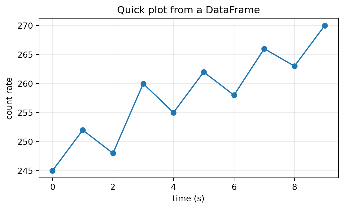

GroupBy basics (quick statistics)

df = pd.DataFrame({
  "shift": ["morning", "morning", "afternoon", "afternoon", "night", "night"],
  "count_rate": [248, 255, 232, 238, 261, 257]
})

summary = df.groupby("shift")["count_rate"].agg(["mean", "std", "count"])
summary

	mean	std	count
shift
afternoon	235.0	4.242641	2
morning	251.5	4.949747	2
night	259.0	2.828427	2

Read CSV

data_path = "data/data_rate_vs_thickness_pb.csv"

df = pd.read_csv(
  data_path,
  comment="#",
  header=None,
  names=["thickness_mm", "count_rate"]
)

df["net_count_rate"] = df["count_rate"] - 50
df.head()

	thickness_mm	count_rate	net_count_rate
0	0	52644	52594
1	3	43823	43773
2	6	35922	35872
3	9	29968	29918
4	12	24771	24721

Write CSV

out_path = "output/day5_pb_with_net.csv"
df.to_csv(out_path, index=False)

print(f"written to: {out_path}")
print("preview of the exported file:")
pd.read_csv(out_path).head()

written to: output/day5_pb_with_net.csv
preview of the exported file:

	thickness_mm	count_rate	net_count_rate
0	0	52644	52594
1	3	43823	43773
2	6	35922	35872
3	9	29968	29918
4	12	24771	24721

index=False avoids writing the pandas row index as an extra column

Pendulum Experiment

We measure the period of a pendulum for different lengths.

Load the dataset:

https://www.physi.uni-heidelberg.de/~reygers/lectures/2026/AI-assisted-Python-Coding/data/pendulum.csv

import pandas as pd

url = "https://www.physi.uni-heidelberg.de/~reygers/lectures/2026/AI-assisted-Python-Coding/data/pendulum.csv"
pendulum_df = pd.read_csv(url)

Tasks:

Load the dataset into a pandas DataFrame and inspect it with head(), shape, and columns.
Create a new column T_squared = period_s**2.
Plot T_squared versus length_m.
Use the relation \(T^2 = \frac{4\pi^2}{g} l\) to estimate \(g\) from the slope of the graph.

Iris scatter plot

We use the public iris dataset from the seaborn example repository:

https://raw.githubusercontent.com/mwaskom/seaborn-data/master/iris.csv

import pandas as pd

url = "https://raw.githubusercontent.com/mwaskom/seaborn-data/master/iris.csv"
iris_df = pd.read_csv(url)

Create a scatter plot similar to the classic iris example from scikit-learn.

Load the dataset into a DataFrame iris_df.
Plot sepal_length on the x-axis and sepal_width on the y-axis.
Show the three species in different colors.
Add axis labels and a legend.
From the plot, describe which species is easiest to separate and which two still overlap.

Very short scikit-learn example

scikit-learn is a standard library for machine learning in Python.

Typical workflow:

load data
split into train/test
choose a model
train and evaluate

Iris dataset: variables

Goal: predict the Iris flower class from measured observables.

The Iris dataset has 3 classes: setosa, versicolor, or virginica

The measured observables are:

sepal length
sepal width
petal length
petal width

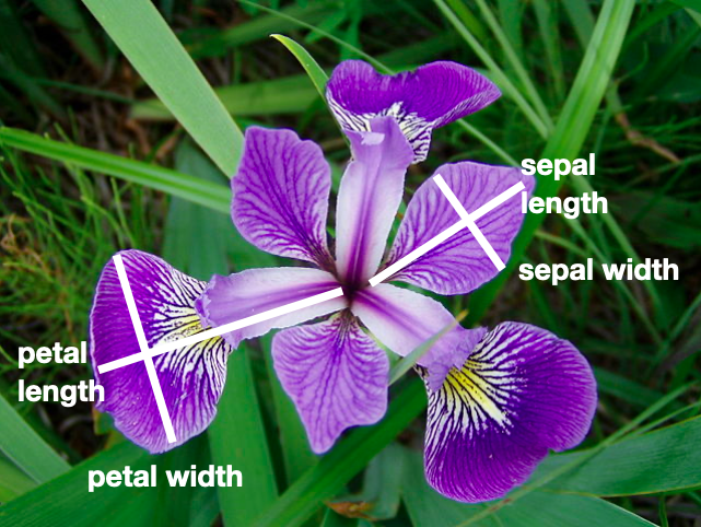
These observables are the input for the classifier.

Load Iris data

from sklearn.datasets import load_iris

iris = load_iris()
X = iris.data
y = iris.target

X.shape, y.shape, iris.target_names, iris.feature_names

((150, 4),
 (150,),
 array(['setosa', 'versicolor', 'virginica'], dtype='<U10'),
 ['sepal length (cm)',
  'sepal width (cm)',
  'petal length (cm)',
  'petal width (cm)'])

Classification with a Multi-Layer Perceptron (MLP)

from sklearn.model_selection import train_test_split
from sklearn.pipeline import make_pipeline
from sklearn.preprocessing import StandardScaler
from sklearn.neural_network import MLPClassifier

X_train, X_test, y_train, y_test = train_test_split(
  X, y, test_size=0.3, random_state=42, stratify=y
)

clf = make_pipeline(
  StandardScaler(),
  MLPClassifier(hidden_layer_sizes=(20,), max_iter=2000, random_state=42)
)

clf.fit(X_train, y_train)
accuracy = clf.score(X_test, y_test)

print(f"test accuracy = {accuracy:.3f}")

test accuracy = 0.933

Evaluate predictions

from sklearn.metrics import confusion_matrix, classification_report

y_pred = clf.predict(X_test)

print("Confusion matrix:")
print(confusion_matrix(y_test, y_pred))

print("\nClassification report:")
print(classification_report(y_test, y_pred, target_names=iris.target_names))

Confusion matrix:
[[15  0  0]
 [ 0 14  1]
 [ 0  2 13]]

Classification report:
              precision    recall  f1-score   support

      setosa       1.00      1.00      1.00        15
  versicolor       0.88      0.93      0.90        15
   virginica       0.93      0.87      0.90        15

    accuracy                           0.93        45
   macro avg       0.93      0.93      0.93        45
weighted avg       0.93      0.93      0.93        45

Exercise: compare classifiers

Continue with the same iris dataset and the same train/test split.

Train two additional classifiers:

KNeighborsClassifier
RandomForestClassifier

Tasks:

Train both models on the training data.
Compute the test accuracy for each model.
Compute a confusion matrix for each model.
Compare the results with the MLP example.
Decide which classifier you would choose for this dataset.

Clean code in scientific Python

Why it matters:

easier to debug and verify results
easier to hand over to lab partners
easier to reuse in reports and papers

Focus today:

KISS
YAGNI
DRY
single responsibility

KISS principle

KISS: Keep It Simple, Stupid.

Use the simplest solution that solves the problem well.

In practice:

clear names (thickness_mm, not t1)
small functions with one task
avoid clever one-liners when a clear 3-line version is better

Reference: KISS principle

YAGNI

YAGNI: You Ain’t Gonna Need It.

Do not implement features before they are needed.

In practice:

avoid “future-proof” abstractions too early
start with a direct script, then refactor when repetition appears
remove dead code and unused options

Reference: YAGNI

DRY

DRY: Don’t Repeat Yourself.

Avoid copying the same logic into several places.

In practice:

if the same code appears 2-3 times, consider a small function
keep constants in one place instead of repeating numbers
copy-paste is fine once, but not as a long-term solution

Reference: DRY principle

Single responsibility

One function or code block should have one clear job.

In practice:

separate loading, analysis, and plotting when possible
prefer load_data(), fit_model(), make_plot() over one long function
this makes testing and debugging much easier

Minimal Git workflow

One-time setup:

Clone a remote repository to your machine and create a local working copy.

git clone <repo-url>

Most common day-to-day commands:

git status
git pull
git add .
git commit -m "Add data analysis for day5"
git push

Helpful safety command:

Discard local changes in a file, or with --staged remove it from the staging area.

git restore <file>

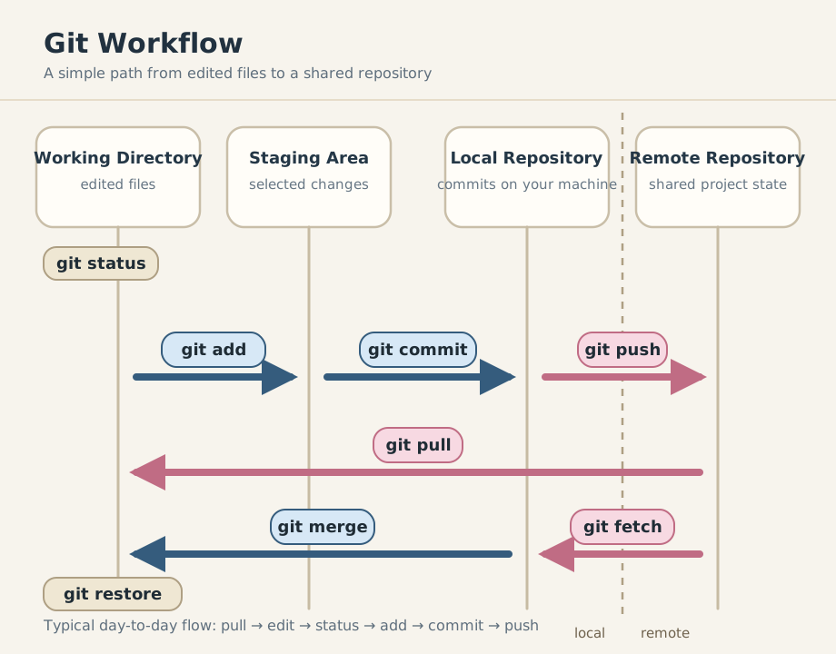
Use small, frequent commits with meaningful messages.

Prompting for code

Useful rule:

give enough context to act
keep the task narrow

Better than:

“Improve my project”

Better:

“In analysis.py, fix the CSV loading error. Keep the function signature unchanged.”
include the relevant code snippet
show expected input/output

Reference: OpenAI Codex Prompting Guide

Prompting: scope and constraints

Good prompts often specify:

file or function
exact bug or feature
relevant code
what must stay unchanged
desired output format

Useful constraints:

keep the public API unchanged
do not add new dependencies
only change one file
prefer minimal changes

Prompting: ask for verification

One of the most useful additions is:

ask the model to check whether the solution actually works

For example:

fix the bug and run the tests
if you cannot run the tests, say what should be tested
add one small test case
compare two implementations and recommend one
explain possible failure cases

This often gives much better answers than just:

“write the code”

Prompting: iterate, do not restart

The first prompt does not need to be perfect.

Often the best workflow is:

prompt 1: solve the main task
prompt 2: simplify or explain
prompt 3: add checks, tests, or polish

Useful follow-up prompts:

make the solution shorter
keep the same behavior but improve readability
suggest a better prompt for this task

For more complex tasks:

first outline a short plan, then implement

Prompting patterns that work well

Reusable prompt patterns:

“fix this bug and explain briefly why it works”
“refactor this code without changing behavior”
“review this code and list possible issues”
“write tests for this function”
“compare these two implementations and recommend one”

These patterns often work better than:

vague or open-ended requests

Coding with AI

treat AI as a collaborator, not a magic tool
prompting = specifying tasks clearly
always verify outputs
work iteratively, not in one shot

AI-assisted Python Coding

Very short introduction to pandas

Core objects: Series and DataFrame

Create and inspect a DataFrame

Select rows and columns

Add columns and filter data

loc and iloc

Quick statistics and sorting

Missing data basics

Plot directly from pandas

GroupBy basics (quick statistics)

Read CSV

Write CSV

Pendulum Experiment

Iris scatter plot

Very short scikit-learn example

Iris dataset: variables

Load Iris data

Classification with a Multi-Layer Perceptron (MLP)

Evaluate predictions

Exercise: compare classifiers

Clean code in scientific Python

KISS principle

YAGNI

DRY

Single responsibility

Minimal Git workflow

Prompting for code

Prompting: scope and constraints

Prompting: ask for verification

Prompting: iterate, do not restart

Prompting patterns that work well

Coding with AI

`loc` and `iloc`