import numpy as np
import matplotlib.pyplot as plt
from scipy.stats import chi2

x = np.linspace(0, 30, 600)
pdf_k5 = chi2.pdf(x, df=5)
pdf_k10 = chi2.pdf(x, df=10)
pdf_k20 = chi2.pdf(x, df=20)

plt.figure(figsize=(6.5, 4.0))
plt.plot(x, pdf_k5, color="tab:blue", linewidth=2, label="df = 5")
plt.plot(x, pdf_k10, color="darkorange", linewidth=2, label="df = 10")
plt.plot(x, pdf_k20, color="tab:green", linewidth=2, label="df = 20")
plt.xlabel(r"$\chi^2$")
plt.ylabel("pdf")
plt.title(r"Chi-square distribution (used in $\chi^2$ fitting)")
plt.grid(True, alpha=0.25)
plt.legend()
plt.show()AI-assisted Python Coding
Day 4: SciPy and SymPy
Klaus Reygers
Studierendentage Physik, Uni Heidelberg, 23.-27.03.2026
Day 4: Introduction to SciPy
- SciPy extends NumPy with scientific algorithms
- Special functions, root finding, integration, and fitting
- Goal: learn when SciPy becomes useful beyond plain NumPy
What is SciPy?
NumPy gives us arrays.
SciPy builds on top of NumPy and adds ready-to-use numerical tools for:
- special functions
- optimization and root finding
- integration and differential equations
- interpolation and signal processing
- statistics and fitting
Rule of thumb:
- Use NumPy for arrays and basic math
- Use SciPy when you need a scientific algorithm
Example: a special function
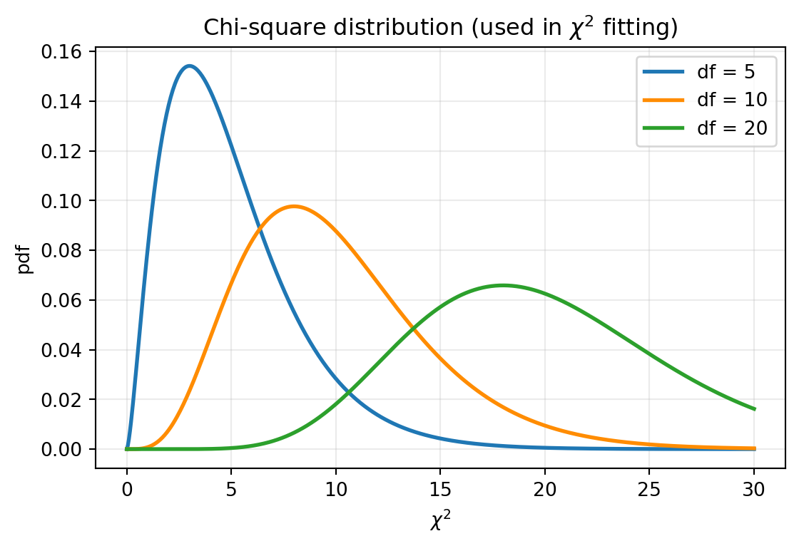
The \(\chi^2\) distribution is defined as the distribution of
\[ Q = \sum_{k=1}^{n} Z_k^2, \qquad Z_k \sim \mathcal{N}(0,1), \]
i.e. the sum of squares of \(n\) independent standard normal random variables.
In data analysis, the chi-square statistic is central for model fitting:
\[ \chi^2 = \sum_i \frac{\left(y_i - f(x_i;\theta)\right)^2}{\sigma_i^2} \]
For Gaussian errors, goodness-of-fit is interpreted with the \(\chi^2\) distribution.
SciPy provides it as scipy.stats.chi2.
Plotting the chi-square distribution
Chi-square distribution: example plot
Physics constants in SciPy
SciPy provides many physical constants in scipy.constants, so you do not need to type them manually.
| Quantity | SciPy name | Value (SI) |
|---|---|---|
| Speed of light \(c\) |
c
|
\(2.99792458 \times 10^8\) m/s |
| Planck constant \(h\) |
h
|
\(6.62607015 \times 10^{-34}\) J s |
| Boltzmann constant \(k_B\) |
k
|
\(1.380649 \times 10^{-23}\) J/K |
| Elementary charge \(e\) |
e
|
\(1.602176634 \times 10^{-19}\) C |
| Avogadro constant \(N_A\) |
N_A
|
\(6.02214076 \times 10^{23}\) 1/mol |
| Vacuum permittivity \(\varepsilon_0\) |
epsilon_0
|
\(8.8541878128 \times 10^{-12}\) F/m |
| Gravitational constant \(G\) |
G
|
\(6.67430 \times 10^{-11}\) m\(^3\) kg\(^{-1}\) s\(^{-2}\) |
Typical usage:
Numerical root finding
SciPy provides several root-finding algorithms in scipy.optimize.
For 1D problems, a common and robust approach is a bracketing method. In practice, Brent’s algorithm (brentq) is often an excellent default choice:
- choose an interval
[a, b] - require that
f(a)andf(b)have opposite signs - then a root is guaranteed somewhere inside the interval
- Brent’s method combines bisection with faster interpolation steps
So in practice, root finding often starts with inspecting the function and choosing a sensible interval.
The mathematical task is still:
\[ f(x) = 0 \]
Root-finding methods
Bisection
- halve the interval \([a,b]\) where \(f(a)\cdot f(b)<0\) repeatedly
- guaranteed to converge, but slow (linear convergence)
Newton’s method
- update: \(x_{n+1} = x_n - f(x_n)/f'(x_n)\)
- very fast near the root, but requires \(f'\) and a good starting point
Secant method
- like Newton, but approximates \(f'\) from two previous function values — no derivative needed
- faster than bisection, but not guaranteed to converge
Brent’s method (brentq) — best of all worlds
- combines bisection (safe) with interpolation/secant steps (fast)
- no derivative needed; guaranteed to converge if a bracket is provided
- in practice: often the best default choice for 1D root finding
Root finding example
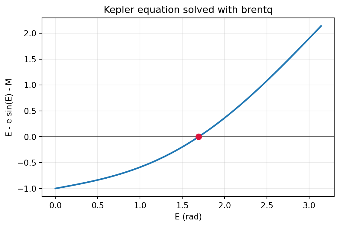
Canonical example from orbital mechanics: Kepler’s equation
\[ f(E) = E - e\sin E - M = 0 \]
with:
- \(M\): mean anomaly
- \(e\): eccentricity
- \(E\): eccentric anomaly (unknown)
This equation is transcendental, so we solve it numerically.
For this example we use \(e = 0.7\), \(M = 1.0\) rad, and bracket \(E \in [0, \pi]\).
Root finding example: solve with brentq
Root finding: visualize the root
Next, we plot the Kepler function
\[ f(E) = E - e\sin E - M \]
and mark the numerical root found by brentq.
One root, one bracket
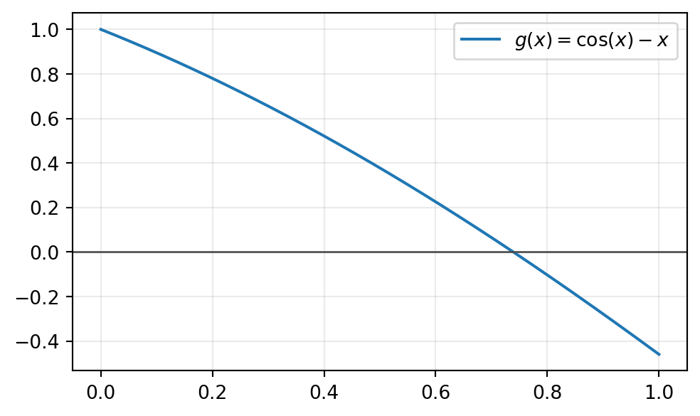
Find the root of
\[ g(x) = \cos(x) - x \]
on the interval \([0, 1]\).
Tasks:
- Plot \(g(x)\) on \([0,1]\) and check the sign change.
- Use
brentqto compute the root. - Compare the execution time of
brentqandbisectfor this problem.
SciPy docs for bisect: https://docs.scipy.org/doc/scipy/reference/generated/scipy.optimize.bisect.html
Solution: one root, one bracket
from time import perf_counter
from scipy.optimize import brentq, bisect

def g(x):
  return np.cos(x) - x

x_brentq = brentq(g, 0.0, 1.0)
x_bisect = bisect(g, 0.0, 1.0)

print(f"brentq root: {x_brentq:.10f}")
print(f"bisect root: {x_bisect:.10f}")
print(f"|g(root)| with brentq: {abs(g(x_brentq)):.2e}")

# 2) Compare runtime
n_runs = 5000

t0 = perf_counter()
for _ in range(n_runs):
  brentq(g, 0.0, 1.0)
t_brentq = perf_counter() - t0

t0 = perf_counter()
for _ in range(n_runs):
  bisect(g, 0.0, 1.0)
t_bisect = perf_counter() - t0

print(f"brentq time for {n_runs} runs: {t_brentq:.4f} s")
print(f"bisect time for {n_runs} runs: {t_bisect:.4f} s")
print(f"speedup (bisect/brentq): {t_bisect / t_brentq:.2f}x")
brentq root: 0.7390851332
bisect root: 0.7390851332
|g(root)| with brentq: 7.88e-15
brentq time for 5000 runs: 0.0501 s
bisect time for 5000 runs: 0.2302 s
speedup (bisect/brentq): 4.60xSolution: plot of \(g(x)=\cos(x)-x\)
Interlude: lambda functions
A lambda function is a short inline function: lambda x: expression.
Why useful:
- concise for one-off functions passed into numerical routines
- keeps code local when a helper is used only once
Rule of thumb: use lambda for simple expressions; use def for longer logic.
Example:
Numerical integration
Core idea: replace a continuous integral by a weighted sum.
\[ \int_a^b f(x)\,dx \approx \sum_{i=1}^{N} w_i f(x_i) \]
Basic principles:
- choose sample points \(x_i\) and weights \(w_i\) (rectangle / trapezoid / Simpson)
- smaller step size usually improves accuracy, but increases compute time
- numerical error must be estimated and controlled
- adaptive methods refine the grid where the function changes rapidly
In practice, scipy.integrate provides these ideas in ready-to-use algorithms.
1D integration example
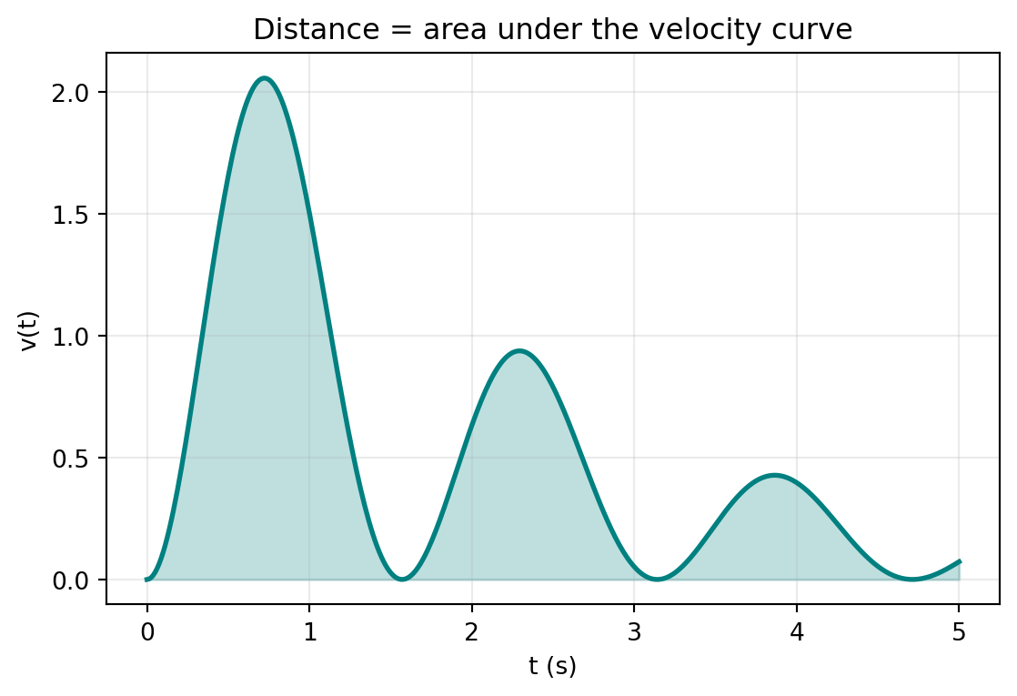
Suppose a particle has velocity
\[ v(t) = 3 e^{-t/2} \sin^2(2t) \]
We compute the distance traveled from \(t=0\) to \(t=5\,\mathrm{s}\).
distance = 2.681467 m
estimated integration error = 7.23e-13
1D integration: visualize the area
1D integration with extra arguments
Consider the Gaussian-like function
\[ f(x; a,b,c) = a \exp\!\left(-\left(\frac{x-b}{c}\right)^2\right). \]
Use scipy.integrate.quad to compute
\[ I = \int_{-1}^{1} f(x; a,b,c)\,dx \]
for \(a=1\), \(b=2\), and \(c=3\).
- Define the function
f(x, a, b, c)in Python. - Read the SciPy documentation for
quadand figure out how extra parameters can be passed to the integrand. - Compute the integral and the estimated integration error.
Solution: 1D integration with extra arguments
integral value = 1.27630684
estimated integration error = 1.42e-14
The key point is args=(1.0, 2.0, 3.0), which passes extra parameters (a, b, c) to f.
2D integration example
Now consider a non-uniform surface charge density
\[ \sigma(x,y) = e^{-(x^2 + y^2)} \]
on the square region \(-1 \le x \le 1\), \(-1 \le y \le 1\).
We want the total charge:
\[ Q = \iint \sigma(x,y)\,dx\,dy \]
2D integration with variable bounds
A pyramid has a triangular base in the \(xy\)-plane:
\[ D = \{(x,y)\mid 0 \le x \le 1,\; 0 \le y \le 1-x\}. \]
The height above point \((x,y)\) is
\[ h(x,y) = H\,(1 - x - y),\qquad H = 1. \]
Compute the volume
\[ V = \iint_D h(x,y)\,dA. \]
- Write the iterated integral with outer variable \(x\) and inner variable \(y\).
- Implement it with
scipy.integrate.dblquad. - Compare your numerical result with the analytic value \(V = 1/6\).
Solution: pyramid volume
\[ V = \int_0^1 \int_0^{1-x} H(1-x-y)\,dy\,dx \]
from scipy.integrate import dblquad

H = 1.0

def height(y, x):
  return H * (1.0 - x - y)

# inner bounds depend on x: y in [0, 1 - x]
V, V_error = dblquad(height, 0.0, 1.0, lambda x: 0.0, lambda x: 1.0 - x)

print(f"V = {V:.6f}")
print(f"estimated integration error = {V_error:.2e}")
print(f"difference to 1/6 = {abs(V - 1/6):.2e}")
V = 0.166667
estimated integration error = 5.53e-15
difference to 1/6 = 2.78e-17The result matches the classical pyramid formula: \(V = \frac{1}{3} \times \text{(base area)} \times \text{(height)} = \frac{1}{3} \times \frac{1}{2} \times 1 = \frac{1}{6}\).
Chi-square fitting
Suppose we measure data points \(\{x_i, y_i\}\) with uncertainties \(\sigma_i\).
For a model \(f(x; \theta)\), the chi-square function is
\[ \chi^2 = \sum_i \frac{\left[y_i - f(x_i; \theta)\right]^2}{\sigma_i^2} \]
Idea:
- small residuals are good
- large uncertainties count less strongly
- the best fit minimizes \(\chi^2\)
Linear vs. non-linear \(\chi^2\) fits
Linear fit: \(y = a x^2 + b x + c\) (example)
- model is linear in parameters \(a\), \(b\), and \(c\)
- \(\chi^2\) as a function of parameters is a paraboloid with one minimum
- parameter errors and covariances follow directly from linear algebra
Non-linear fit: \(y = a e^{-b x} + c\) (example)
- model is non-linear in parameters \(a\), \(b\), and \(c\)
- \(\chi^2\) surface can have multiple local minima
- requires iterative numerical optimization
- initial guess for the parameters matters for convergence
scipy.optimize.curve_fit
scipy.optimize.curve_fit works for both linear and non-linear models.
- provide model function, data, and optionally uncertainties
sigma - for non-linear models, provide a sensible initial guess via
p0 - inspect residuals and parameter uncertainties after fitting
Typical workflow:
- define model \(f(x;\theta)\)
- fit parameters by minimizing \(\chi^2\)
- validate result (residuals, uncertainties, plausibility)
Straight line fit example: the data
We use the five data points from the error-bar example:
(array([1., 2., 3., 4., 5.]),
 array([1.7, 2.3, 3.5, 3.3, 4.3]),
 array([0.5, 0.3, 0.4, 0.4, 0.6]))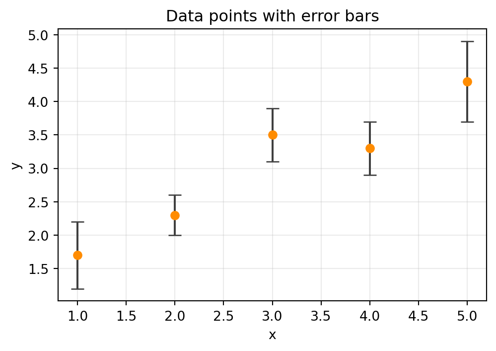
\(\chi^2\) fit
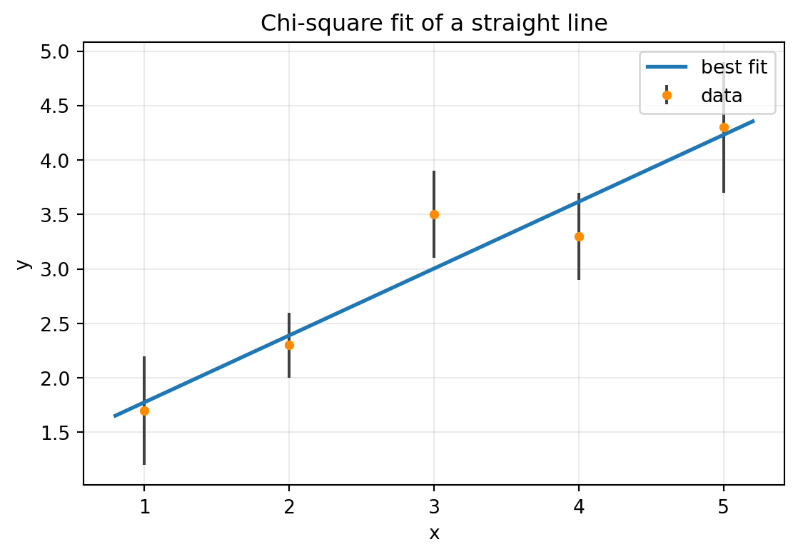
We fit the straight line
\[ y = a x + b \]
with curve_fit using the uncertainties sigma_y.
The fit returns:
- best-fit parameters
a,b - parameter errors
- covariance matrix
from scipy.optimize import curve_fit

def linear_model(x, a, b):
  return a * x + b

popt, pcov = curve_fit(
  linear_model,
  x_data,
  y_data,
  sigma=sigma_y,
  absolute_sigma=True
)

a_fit, b_fit = popt
sigma_a, sigma_b = np.sqrt(np.diag(pcov))

print(f"a = {a_fit:.4f} +/- {sigma_a:.4f}")
print(f"b = {b_fit:.4f} +/- {sigma_b:.4f}")
print("covariance matrix =")
print(pcov)
a = 0.6139 +/- 0.1530
b = 1.1621 +/- 0.4596
covariance matrix =
[[ 0.02341046 -0.06460345]
[-0.06460345 0.2111863 ]]Linear fit: example plot
What do the fit errors mean?
poptcontains the best-fit parameterspcovis the covariance matrix- the parameter errors are the square roots of the diagonal elements:
\[ \sigma_a = \sqrt{(\mathrm{pcov})_{00}}, \qquad \sigma_b = \sqrt{(\mathrm{pcov})_{11}} \]
Off-diagonal entries describe correlations between parameters.
Covariance matrix: definition
For fit parameters \(\theta = (\theta_1, \theta_2, \dots)\), the covariance matrix is
\[ \mathrm{Cov}(\theta)_{ij} = \mathrm{cov}(\theta_i, \theta_j) \]
with
\[ \mathrm{cov}(u,v) = \mathbb{E}\!\left[(u-\mathbb{E}[u])(v-\mathbb{E}[v])\right]. \]
Interpretation:
- diagonal elements: variances, e.g. \(\mathrm{Var}(\theta_i)=\mathrm{Cov}_{ii}\)
- square roots of diagonal elements: 1\(\sigma\) parameter uncertainties
- off-diagonal elements: how strongly parameters change together
In practice with SciPy: pcov[i, i] is the variance of parameter i.
Non-linear fit: gamma attenuation in lead
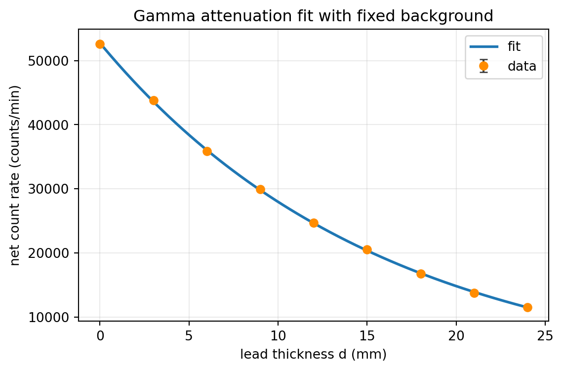
A detector measures the net gamma count rate \(R(d)\) after passing through lead of thickness \(d\). The background has already been subtracted from the data.
Model:
\[ R(d) = R_0 e^{-\mu d} \]
Fit \(R_0\) and \(\mu\). The data points are available here: data/data_rate_vs_thickness_pb_with_net.csv
Tasks:
- Fit the model with
curve_fitto estimate \(R_0\) and \(\mu\). - Determine the half-value layer \(d_{1/2} = \ln(2)/\mu\) from your fit.
- Plot data with error bars and overlay the fitted curve.
Solution: non-linear gamma attenuation
import numpy as np
from scipy.optimize import curve_fit

data = np.genfromtxt("data/data_rate_vs_thickness_pb_with_net.csv", delimiter=",", names=True)

d_data = data["thickness_mm"]
R_data = data["net_count_rate"]
sigma_R = np.sqrt(data["count_rate"])

def attenuation_model(d, R0, mu):
  return R0 * np.exp(-mu * d)

p0 = [R_data[0], 0.05]
popt, pcov = curve_fit(
  attenuation_model,
  d_data,
  R_data,
  sigma=sigma_R,
  absolute_sigma=True,
  p0=p0
)

R0_fit, mu_fit = popt
sigma_R0, sigma_mu = np.sqrt(np.diag(pcov))

d_half = np.log(2.0) / mu_fit
sigma_d_half = np.log(2.0) / (mu_fit**2) * sigma_mu

print(f"R0 = {R0_fit:.1f} +/- {sigma_R0:.1f} counts/min")
print(f"mu = {mu_fit:.4f} +/- {sigma_mu:.4f} 1/mm")
print(f"d_1/2 = {d_half:.2f} +/- {sigma_d_half:.2f} mm")
R0 = 52744.5 +/- 161.8 counts/min
mu = 0.0634 +/- 0.0003 1/mm
d_1/2 = 10.93 +/- 0.05 mmSolution: attenuation fit plot
SciPy summary
scipy.stats: probability distributions such aschi2scipy.optimize: root finding and fittingscipy.integrate: 1D and multi-dimensional integrationcurve_fitreturns both best-fit parameters and the covariance matrix
SciPy becomes especially useful when NumPy arrays are not enough and you need a numerical method.
Introduction to SymPy
SymPy is the symbolic math library in Python.
Use SymPy when you want:
- exact expressions (instead of floating-point approximations)
- algebraic manipulation (simplify, factor, expand)
- analytic derivatives and integrals
- symbolic equation solving
Examples below are adapted from material/intro_sympy.ipynb.
SymPy basics: symbols and exact numbers
(sqrt(2), 1.41421356237309504880168872421)sp.S(1)/2 keeps the value exact as a SymPy rational number.
Expression manipulation
(1, sin(2*x), (x + 1)**2)Typical workflow:
- build an expression
- simplify it
- inspect mathematically equivalent forms
Symbolic differentiation
\(\displaystyle e^{x} \sin{\left(x \right)} + e^{x} \cos{\left(x \right)}\)
You can also compute higher derivatives:
Taylor expansion with series
SymPy can compute Taylor expansions symbolically:
sin(x) around x=0: x - x**3/6 + x**5/120 + O(x**7)
polynomial part: x**5/120 - x**3/6 + x
Small-angle physics approximation (for x << 1):
\(\displaystyle x - \frac{x^{3}}{6} + O\left(x^{5}\right)\)
This gives \(\sin x \approx x - x^3/6\) to third order.
Symbolic integration
Indefinite integral:
\(\displaystyle e^{x} \sin{\left(x \right)}\)
Definite integral:
Solving equations
Single equation:
System of equations:
Substitution
subs is very useful to evaluate symbolic expressions at specific values.
Change of variables and Jacobian
Example: spherical coordinates transformation.
\(\displaystyle r^{2} \sin{\left(\theta \right)}\)
The Jacobian determinant appears in coordinate transformations and volume elements.
Solving differential equations symbolically
\(\displaystyle f{\left(x \right)} = C_{1} \sin{\left(x \right)} + C_{2} \cos{\left(x \right)}\)
Another example with forcing:
From symbolic to numeric (lambdify)
SymPy expressions can be converted to fast NumPy-callable functions.
array([ 0.        ,  0.60294031,  0.46684887,  0.05191515, -0.19949097,
       -0.1811174 ])
This is a common bridge from symbolic derivation to numerical simulation/plotting.
Gaussian error propagation
For a function \(f(x_1, x_2, \ldots, x_n)\) with uncorrelated variables, each measured with uncertainty \(\sigma_{x_i}\):
\[ \sigma_f = \sqrt{\sum_{i=1}^{n} \left(\frac{\partial f}{\partial x_i}\right)^2 \sigma_{x_i}^2} \]
- Valid in the linear approximation (first-order Taylor expansion)
- Requires that uncertainties are small compared to the scale on which \(f\) varies
Example: \(z = x \cdot y\)
\[ \sigma_z = \sqrt{(y\,\sigma_x)^2 + (x\,\sigma_y)^2} = z \, \sqrt{\left(\frac{\sigma_x}{x}\right)^2 + \left(\frac{\sigma_y}{y}\right)^2} \]
Gaussian error propagation with SymPy
Pendulum relation:
\[ g = \frac{4\pi^2 l}{T^2} \]
with measured quantities:
- length \(l\) with uncertainty \(\sigma_l\)
- period \(T\) with uncertainty \(\sigma_T\)
\[ \sigma_g = \sqrt{\left(\frac{\partial g}{\partial l}\right)^2\!\sigma_l^2 + \left(\frac{\partial g}{\partial T}\right)^2\!\sigma_T^2} \]
SymPy can compute the partial derivatives and simplify \(\sigma_g\) symbolically.
Symbolic derivation of \(\sigma_g\)
(4*pi**2*l/T**2,
 4*pi**2/T**2,
 -8*pi**2*l/T**3,
4*pi**2*sqrt(T**2*sigma_l**2 + 4*l**2*sigma_T**2)/T**3)Pendulum example with numbers
# Example measurements
vals = {
  l: 1.00,       # m
  T: 2.01,       # s
  sigma_l: 0.005,  # m
  sigma_T: 0.02    # s
}

g_val = g_expr.subs(vals).evalf()
sigma_g_val = sigma_g_expr.subs(vals).evalf()

rel_percent = 100 * sigma_g_val / g_val

print(f"g = {g_val:.4f} m/s^2")
print(f"sigma_g = {sigma_g_val:.4f} m/s^2")
print(f"relative uncertainty = {rel_percent:.2f}%")
g = 9.7716 m/s^2
sigma_g = 0.2005 m/s^2
relative uncertainty = 2.05%A general symbolic error propagation function
Use an LLM to write a function error_propagation(expr, variables, uncertainties) that takes:
- a SymPy expression
exprfor a quantity of interest - a list of SymPy symbols
variablesthat have uncertainties - a list of SymPy symbols
uncertaintiescorresponding to the uncertainties of those variables
The function should return a SymPy expression for the propagated uncertainty of expr using the Gaussian error propagation formula.
Test the function with the pendulum example derivation.
Different error propagation methods
Consider the same pendulum example with \(g = 4\pi^2 l / T^2\). 1. Use your error_propagation function to compute \(\sigma_g\) symbolically. 2. Calculate the uncertainty \(\sigma_g\) using Monte Carlo error propagation: - Generate random samples for \(l\) and \(T\) based on their uncertainties (e.g., using normal distributions). - Compute the distribution of \(g\) from these samples. - Estimate \(\sigma_g\) as the standard deviation of the resulting \(g\) distribution. 3. Install the module uncertainties and use it to determine the uncertainty
Compare results.
SymPy summary
symbols, exact numbers, and algebraic expressionssimplify,trigsimp,factorfor expression manipulationdiff,integrate,solve,dsolvefor core symbolic tasks- Jacobians for coordinate transforms
lambdifyto use symbolic formulas numerically
SymPy is ideal when understanding the form of equations matters, not only numeric values.