Hands-on: the lighthouse problem (another unbinned ML fit)
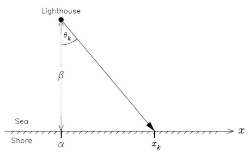
A lighthouse is somewhere off a piece of straight coastline at a position $\alpha$ along the shore and a distance $\beta$ out at sea (see figure). Its lamp rotates with constant velocity but it is not on at all the times: it emits a series of short highly collimated flashes at random intervals and hence at random angles $\theta_k$. These pulses are intercepted on the coast by photo-detectors that record only the fact that a flash has occurred, but not the angle from which it came. $N = 1000$ flashes have so far been recorded with positions $x_k$.
Our goal is to estimate the lighthouse position using the likelihood method.
This problem is discussed, e.g., in Sivia, Skilling, "Data Analysis: A Bayesian Tutorial".
Elementary geometry allows us to write
$$x_k(\theta_k) = \alpha + \beta\tan\theta_k$$The angle $\theta$ is uniformly distributed between $-\pi/2$ and $\pi/2$. We obtain the pdf $p(x | \alpha, \beta)$ from a change of variables:
$$p(x | \alpha, \beta) = f(\theta(x))\left|\frac{d\theta}{dx}\right|, \quad f(\theta) = const.$$$$\theta(x) = \tan^{-1}\left(\frac{x-\alpha}{\beta}\right), \quad \frac{d\theta}{dx} = \frac{\beta}{(x - \alpha)^2 + \beta^2}$$In summary, the normalized pdf for measuring the light flash at position $x$ for given values $\alpha$ and $\beta$ is given by
$$ p(x | \alpha, \beta) = \frac{1}{\pi}\frac{\beta}{(x - \alpha)^2 + \beta^2} $$This is known as Cauchy distribution, a distribution which neither has a mean nor a variance as the corresponding integrals diverge.
# Load the data on the recorded positions and plot their distribution as an histogram.
import pandas as pd
d = pd.read_csv('../data/lighthouse.csv')
# plot the data
import matplotlib.pyplot as plt
plt.hist(d['xk'], bins=50, range=(-500, 500), histtype='step');

a) Define a python function that takes as input the values of $x_k$ (as a numpy array) and the parameters $\alpha$ and $\beta$ and returns the corresponding values of the probability density function.
import numpy as np
def p(x, alpha, beta):
    ### begin solution

    # your code here

    ### end solution
    return pdf_val
b) Now we would like to visualize the likelihood function for a given (small) number $n$ of measurements $x_k$. In the Bayesian view this is the posterior distribution. Plot the posterior distribution in a 2 x 2 panel plot for $n = 1, 2, 10, 50$.
def Ltmp(alpha, n):
    # n = number of data points (we arbitrarily start at data point 300)
    beta = 30
    pv = p(d['xk'][300:300+n], alpha, beta)
    return np.prod(pv)
L = np.vectorize(Ltmp) # make it usable for numpay arrays
# your code here

# fig, axes = plt.subplots(nrows=2, ncols=2)
# fig.tight_layout()

# av = np.linspace(-100., 100., 100)
# plt.subplot(2, 2, 1)
# plt.plot(av, L(av, 1), label='n = 1')
# plt.legend()

# ...
c) Now write a python function that returns the logarithm of the likelihood of the given dataset as a function of $\alpha$ and $\beta$.
def LL(alpha, beta):
    ### begin solution

    # your code here
    # data: d['xk']

    ### end solution
    return LogLikelihood

def NLL(alpha, beta):
    return -LL(alpha, beta)
d) Now we want to find the values of $\alpha$ and $\beta$ for which the logarithm of the likelihood is maximised. To do that we can use the migrad numerical minimiser from the package iminuit. Since this looks for the minimum rather than the maximum of the given function we will pass to it the negative logarithm of the likelihood NLL (defined by multiplying the logarithm of the likelihood by -1).
The basic usage of Minuit is described here: https://nbviewer.jupyter.org/github/scikit-hep/iminuit/blob/master/tutorial/basic_tutorial.ipynb
from iminuit import Minuit

# your code here
e) Plot the fitted pdf along with the data
xs=np.linspace(-200,200,400)
plt.hist(d['xk'], bins=200, density=True, histtype='step', range=(-1000,1000));
plt.xlim(-200, 200);

# your code here
